Quick Access
 O(1)
O(1)
 O(log n)
 O(n)
O(n)
 O(n log n)
 O(n2)
O(n2)
 O(2n)
O(2n)
 O(n!)
O(n!)
 Maths
Maths
Introduction
Everything on a computer relies in some way on some algorithms. Every algorithm takes time and space to execute. The complexity of that code is an estimation of this time/space for its execution. The lesser the complexity, the better the execution.
The complexity, or Big O notation, then allow us to be able to compare algorithms without implementing or running them. It helps us to design an efficient algorithm, and that is why any tech interview in the world asks about the running complexity of a program.
The complexity is an estimation of asymptotic behavior. This is a measure of how an algorithm scales, not a measurement of specific performance.
Objectives
Understand how algorithm performances are calculated. Estimate the time or space requirements of an algorithm. Identify the complexity of a function. Keep in mind that Big O is an asymptotic measure and stays a fuzzy lens into performance.
What is next?
You will then be much more confident going further with more complex data structures (binary tree, hash map, etc.) and explore some algorithm implementations such as sorting or maze generators.
Common Running Times
Here is a general picture of the standard running times used when analyzing an algorithm : it is a great picture to keep in mind each time we write some code.
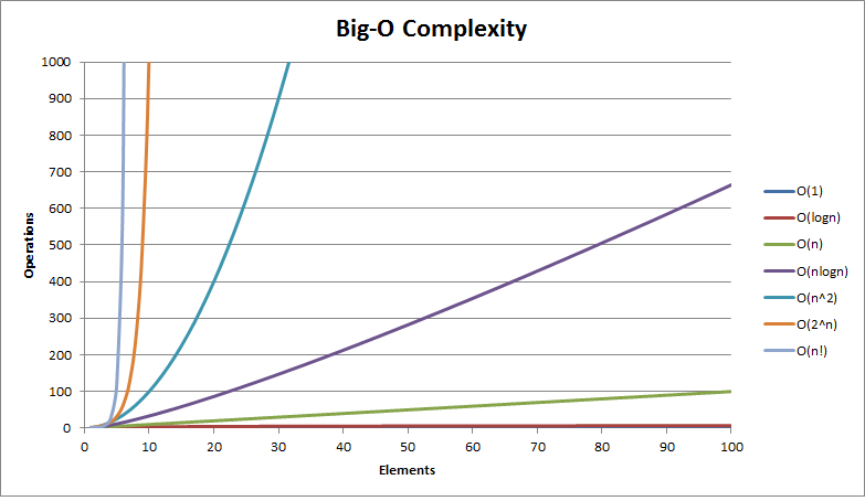
The graph above shows the number of operations performed by an algorithm against the number of input elements. It can be seen how quick its complexity may penalize an algorithm.
The complexity that can be achieved depends on the problem. Let us see below ordinary running times and some corresponding algorithm implementations.
Constant - O(1)
Constant time means the running time is constant : it is like as fast as the light whatever the input size is! It concerns for instance most of the basic operations you may have with any programming language (e.g. assignment, arithmetic, comparisons, accessing array’s elements, swap values...).
auto a = -1;                    // O(1)
auto b = 1 + 3 * 4 + (6 / 5);   // O(1)
auto d = swap(a, b);            // O(1)

if (a < b)
  auto c = new Object();        // O(1)

auto array = {1, 2, 3, 4, 6};   // O(1)
auto i = array[4];              // O(1)
...
Logarithmic - O(log n)
Those are the fastest kind of algorithms complexity that depends on the data input size. The most well-known and easy to understand algorithm showing this complexity is the binary search which code is shown below.
Index BinarySearch(Iterator begin, Iterator end, const T key)
{
  auto index = -1;
  auto middle = begin + distance(begin, end) / 2;

  // While there is still objects between the two iterators and no object has been found yet
  while(begin < end && index < 0)
  {
    if (IsEqual(key, middle))   // Object Found: Retrieve index
      index = position(middle);
    else if (key > middle)      // Search key within upper sequence
      begin = middle + 1;
    else                        // Search key within lower sequence
      end = middle;

    middle = begin + distance(begin, end) / 2;
  }

  return index;
}
Commonly : divide and conquer algorithms may result in a logarithmic complexity.
Linear - O(n)
The running time increases at most linearly with the size of the input : if the input size is n, it will perform ~n operations as well. Linear time is the best possible time complexity in situations where the algorithm has to read its entire input sequentially.
Consider the example where we have to compute the sum of gains and losses (total gain). For sure, we will have to go through each value at least once:
T Gain(Iterator begin, Iterator end)
{
  auto gain = T(0);
  for (auto it = begin; it != end; ++it)
    gain += *it;

  return gain;
}
If you have a unique for loop with simple data, it most probably results in O(n) complexity.
Quasilinear - O(n log n)
Algorithms with a O(n log n) running time are slightly slower than those in O(n). This is for instance the best time complexity dealing with sorting algorithms.
In many cases, the n log n complexity is simply the result of performing a logarithmic operation n times or vice versa. As example, the classic merge sort algorithm:
void MergeSort(Iterator begin, Iterator end)
{
  const auto size = distance(begin, end);
  if (size < 2)
    return;

  auto pivot = begin + (size / 2);

  // Recursively break the vector into two pieces
  MergeSort(begin, pivot); // O(log n)
  MergeSort(pivot, end);   // O(log n)

  // Merge the two pieces - considered to be in O(n)
  Merge(begin, pivot, end); // O(n)
}
They often are the result of some optimization from a O(n2) algorithm.
Quadratic - O(n2)
This is the kind of consumptive complexity encountered regularly. Those algorithms often arise when we want to compare each element with all of the others. The Bubble sort, one of the first algorithm generally studied in class, illustrate perfectly this running time. Here is its most naive version:
void BubbleSort (Iterator begin, Iterator end)
{
  // For each pair of elements - bubble the greater up.
  for (auto it = begin; it != end; ++it)
    for (auto itB = begin; itB < end; ++itB)
      if (Compare(itB, (itB + 1))) swap(itB, (itB + 1));
}
If you have a double for loop with simple data, it most probably results in O(n2) complexity.
Exponential - O(2n)
Here is the start of the kind of algorithms that are very consumptive. Usually n2 complexity is acceptable while 2n is almost always unacceptable. The naive recursive fibonacci implementation is its most well-known example:
int Fibonacci(int n)
{
    if (n <= 1)
        return 1;

    return Fibonacci(n - 1) + Fibonacci(n - 2);
}
To see how quickly the running time may climb, if you have: - 5 elements --> 32 operations - 10 elements --> 1024 operations - 100 elements --> 1,2676506×10³⁰ operations !
Still, for some problems we cannot achieve a better complexity. This is for instance the case of the traveling salesman problem that can best reach this complexity thanks to dynamic programming optimizations.
Factorial - O(n!)
It's the slowest of them all and is considered impracticable. We mostly wouldn't have to deal with such algorithms.
This is for instance the case of the traveling salesman problem via brute-force search : it tries all permutations and searches using brute-force which one is cheapest.
Math
To avoid being too long and annoy most of the reader, we will only put some useful mathematics equalities as a reminder for those that want to play further with complexity calculation.
| Math Sums | Master Theorem for Divide and Conquer Recurrences |
|---|---|
| $$\sum_{i=0}^{n-1} {C}^{ste} = n * {C}^{ste}$$ | $$T(n) = O(n) + 2T(\frac{n}{2}) --> O(n log n)$$ |
| $$\sum_{i=0}^{n-1} n = n(n-1)$$ | $$T(n) = O(1) + T(\frac{n}{2}) --> O(log n)$$ |
| $$\sum_{i=0}^{n-1} i = \frac{n(n + 1)}{2} - n = \frac{n(n - 1)}{2}$$ | |
| $$\sum_{i=0}^{n-1} (n+i) = \sum_{i=0}^{n-1} n + \sum_{i=0}^{n-1} i$$ |
Asymptotics of the generalized harmonic number Hn,r:
$$H_{n,r} = \sum_{k=1}^{n} \frac{1}{k^r}$$ $$For \quad n \approx 1$$ $$H_{n,1} \in O(log(n))$$