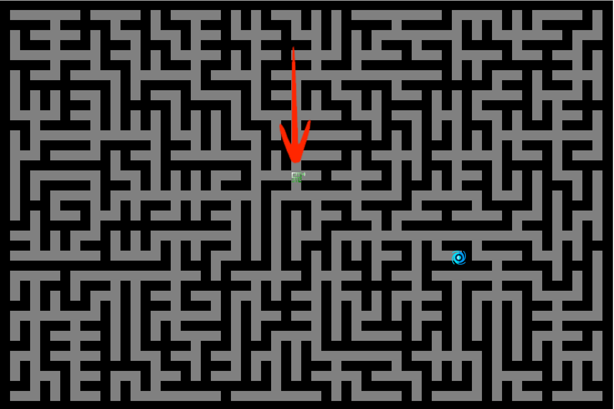
Our board : a random 30x20 maze generated using a Prim's algorithm.
Globo (our green mascot in the middle) is the player and the blue capsule is the goal.

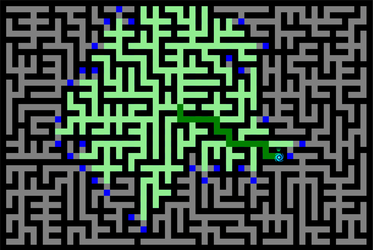
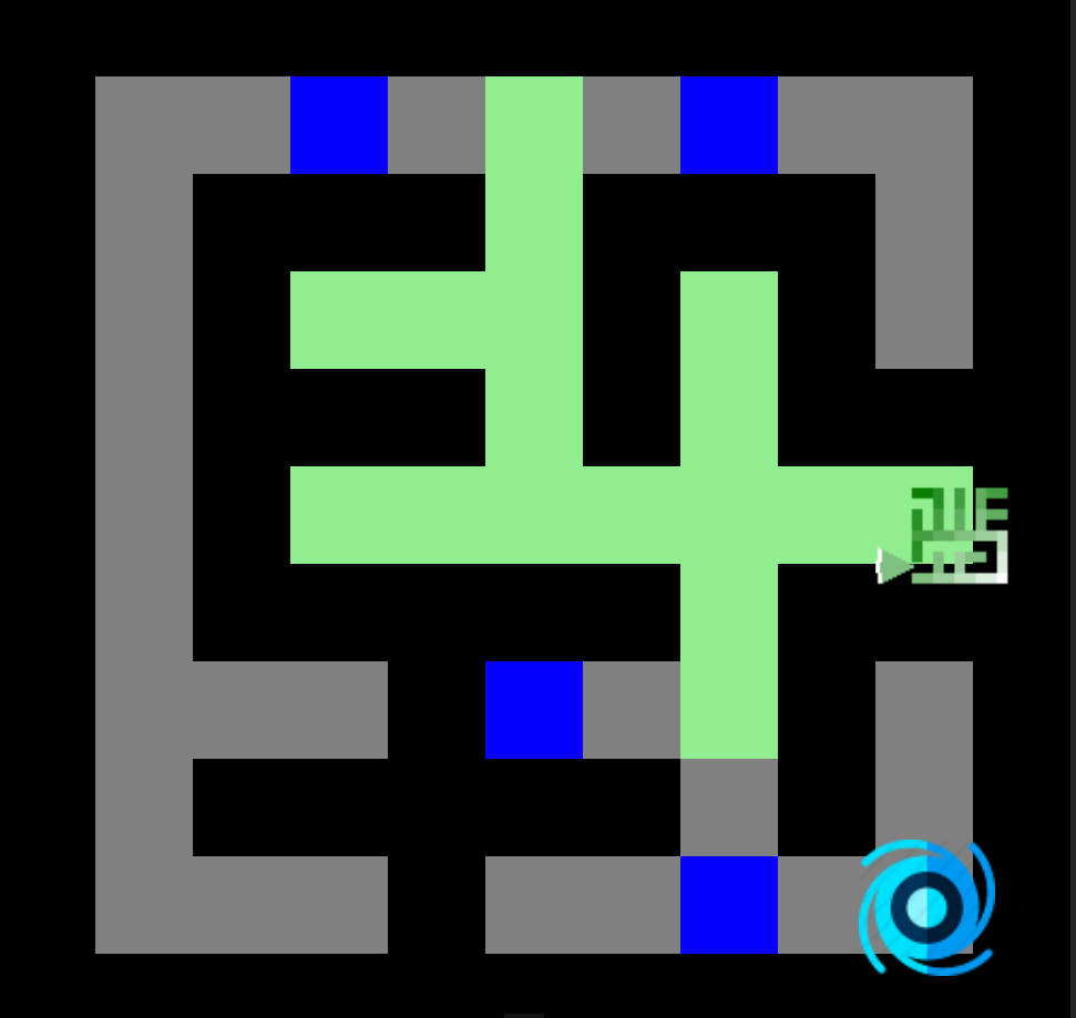
Trace let by the player using Dijkstra's pathfinding algorithm to reach the goal.

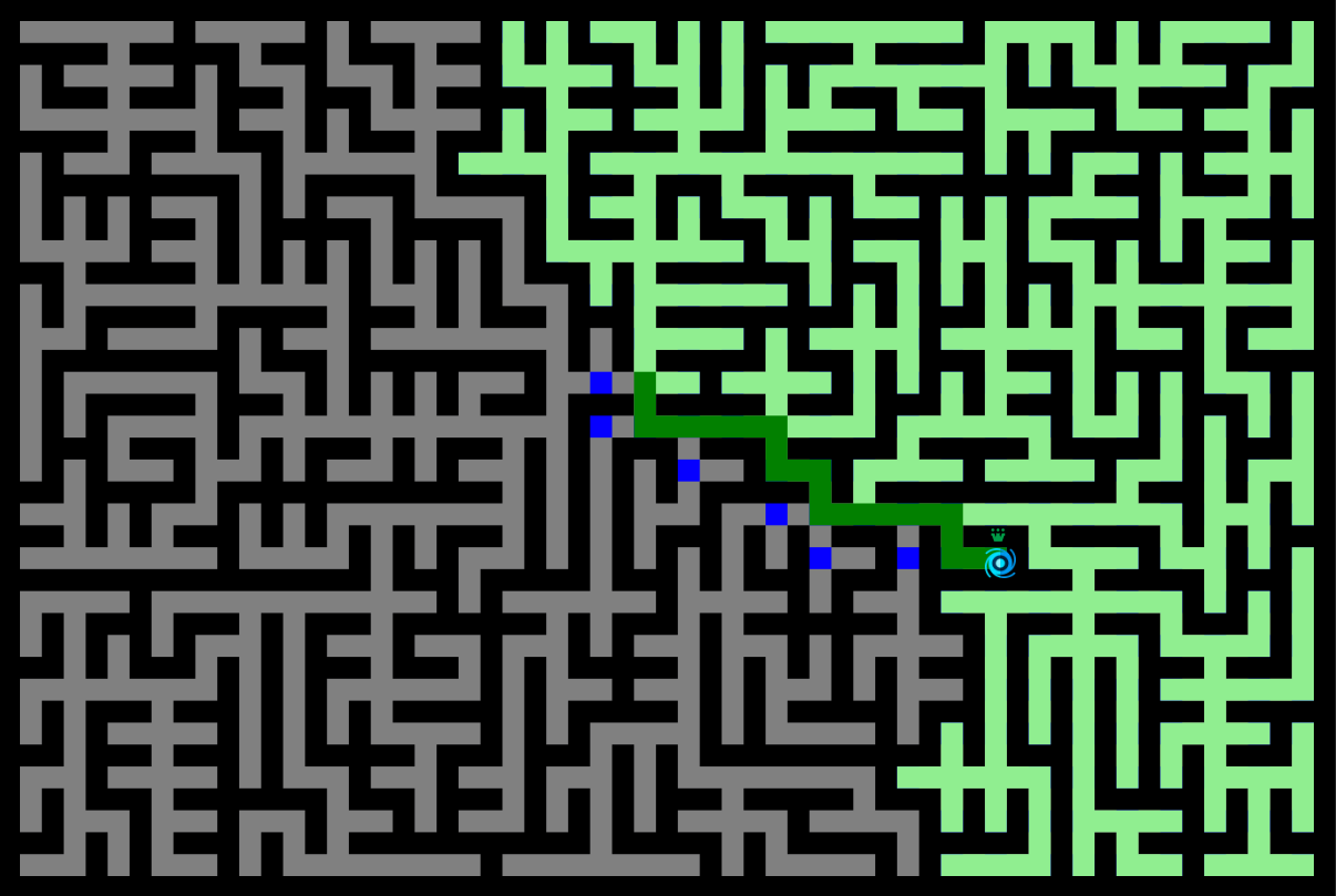
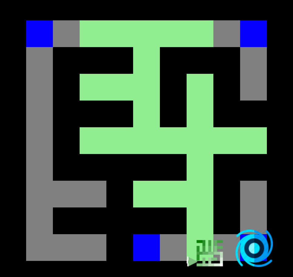
Here is, to be compared, the trace let by the player using a Depth First Search pathfinding algorithm to reach the goal.

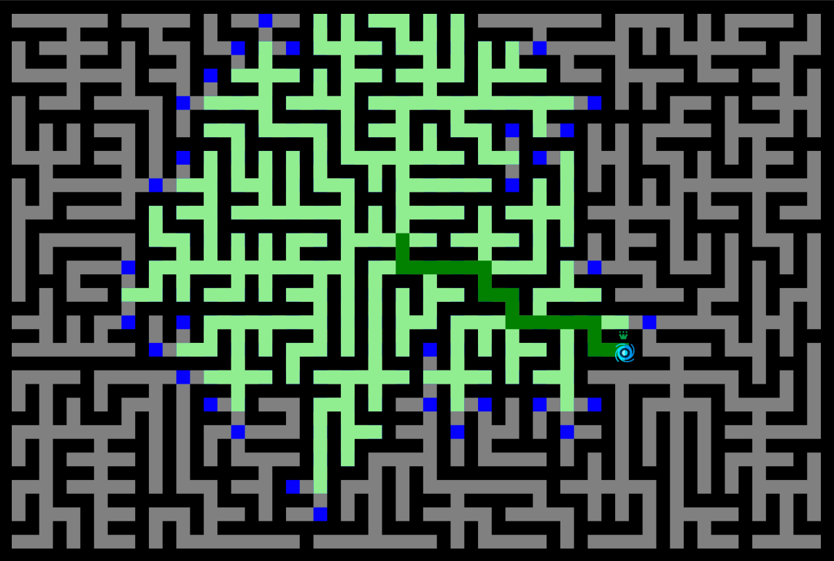
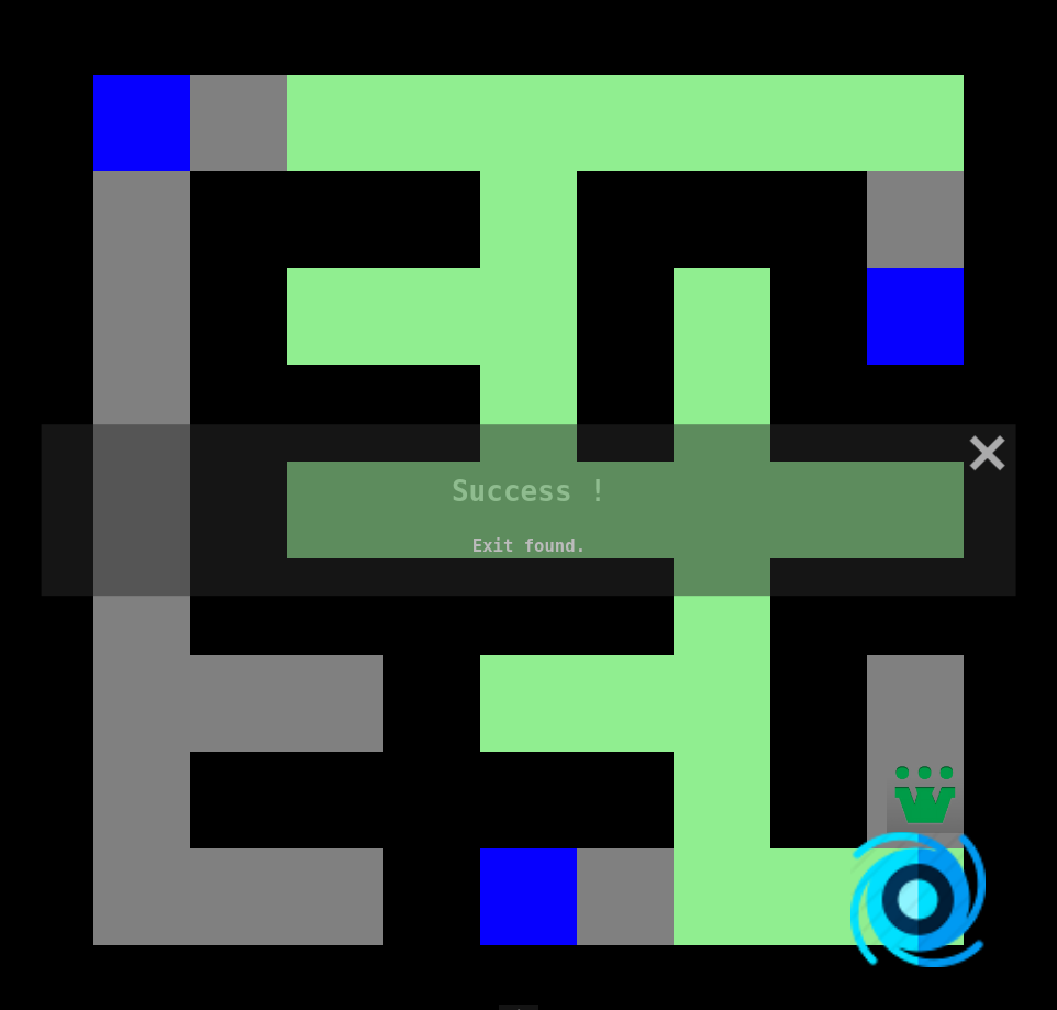
Finally, the trace let by the player using a Breadth First Search (BFS) pathfinding algorithm to reach the goal.

We will see why it is similar to Dijkstra in our case.

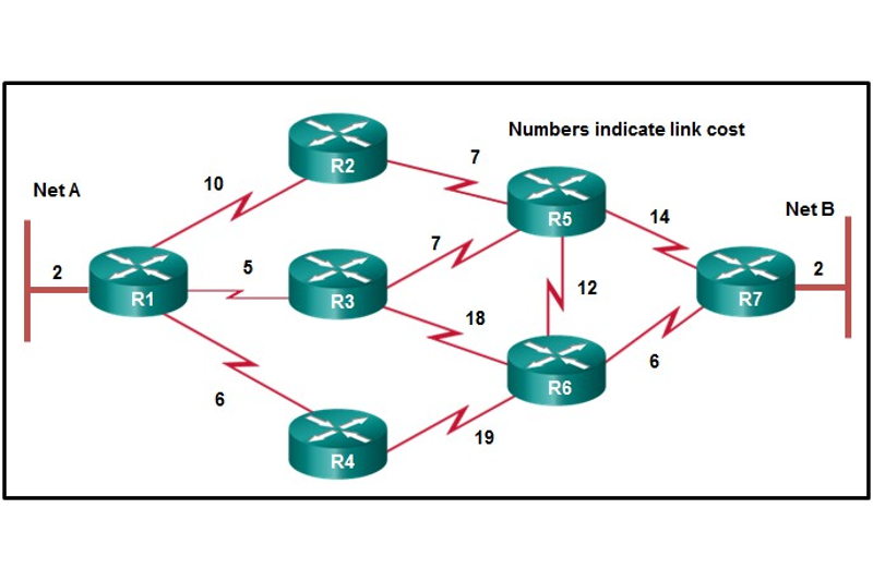
Pathfinding has gained prominence in the early 1950's in the context of routing; that is, finding shortest directions between two or more nodes. In 1956, the Dutch software engineer Edsger Wybe Dijkstra created the best-known of these algorithms : Dijkstra.

Dijkstra’s algorithm finds the shortest path from a root node to every other node (until the target is reached). Dijkstra is one of the most useful graph algorithms; furthermore, it can easily be modified to solve many different problems.

Traversal algorithms such as breadth-first-search and depth-first-search explore all possibilities : they iterate over all possible paths until they reach the target. However, it may not be necessary to examine all possible paths; Dijkstra’s algorithm eliminates useless traversal using heuristics to find the optimal paths.

Some applications

• Widely used in Network routing protocols.
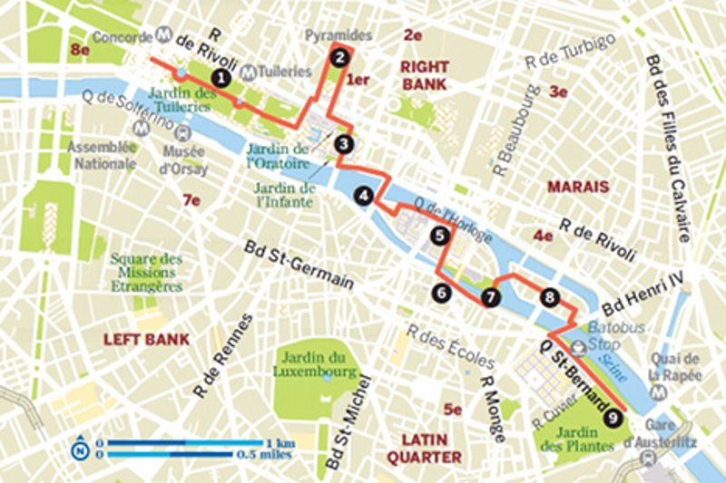
• In digital mapping services such as Google Maps.
• In Biology by finding the network model in spreading of infectious diseases.
• In finding the optimal agenda of flights.
• In path planning for mobile robot transportation...

Used to compute a romantic riverside walk in Paris.

Used to find a network routing.

Used in models such as 'simulating city-level airborne infectious diseases'.

Used to compute flight scheduling.

This algorithm begins with a root (or start) node and a queue of candidate nodes. At each step, we compute minimal distance between the root and each unvisited neighbors. Then, we add them to the queue; the one with the lowest distance is the next one that will be taken from the queue. This process repeats until a path to the destination has been found.

Since the lowest distance nodes are examined first, the first time the destination is found, the path to it will be the shortest path.

Minimizing the distance from the root node is our heuristic here.

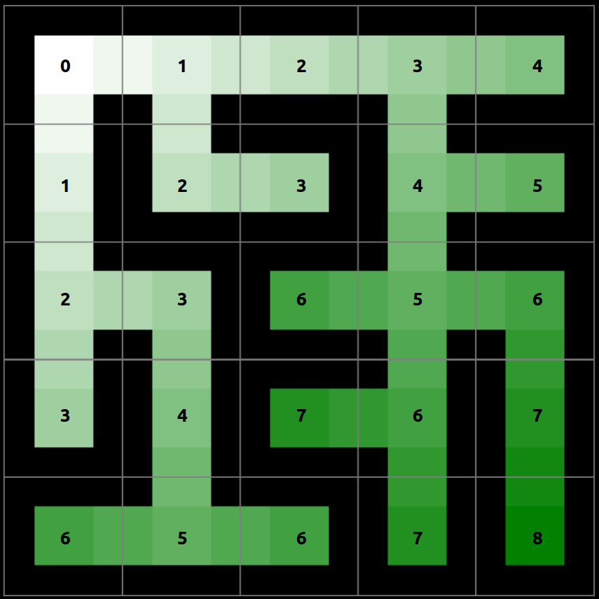
Here is the distance map computed for a maze from the top left corner (root). You may notice that each connection between two adjacent nodes has a distance cost of 1.

Steps

Let's take a root node and note D the distance from a node to the root. Dijkstra's algorithm will assign some initial distance values and improve them step by step.

• 1. Set all node distance D to infinity except for the root (current) node which distance is 0.
• 2. Mark current node as visited and update D for all of its unvisited neighbours with the shortest distance.
  Note: we can stop the algorithm here if we have reached the target node.
• 3. Add to the queue the unvisited neighbours and go back to step 2.

Yes, one of the most useful and used algorithms is as simple as that !

As we have seen : by calculating and continually updating the shortest distance, the algorithm compiles the shortest path to the destination. A key part of this approach is maintaining an ordered line of nodes to visit next; to set up that part of the algorithm, we will use a priority queue (a regular queue with the ability to set priorities).

For Dijkstra’s algorithm, it is always recommended to use priority queue (or heap) as the required operations (extract minimum and decrease key) match with specialty this data structure. Here the priority is defined by D (the distance between a node and the root). Higher priorities are given for nodes with lower distance D.

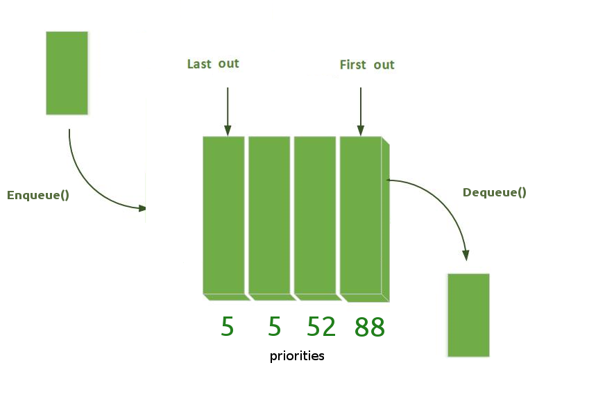
You may see it as a regular attraction queue with some people having access to shortcut heading to different checkpoints. A priority queue should have the following methods:

// Add new element at the end of the queue
void enqueue(const T& data, const int priority);

// Remove element from the beginning of the queue
void dequeue();

// Change the priority of the element in the queue.
void changePriority(const T& item, const int priority);

Now that we know all we need to know, here is the implementation (the visual explanation follows):

Code

Dijkstra(Maze maze, Node start, Node end) {
    priority_queue queue();

    // Init all distances with infinity
    for (auto&& node : maze.nodes) node.distance = Infinity;

    // Distance to the root itself is zero
    start.distance = 0;

    // Init queue with the root node
    queue.add(start, 0);

    // Iterate over the priority queue until it is empty.
    while (!queue.isEmpty()) {
      curNode = queue.dequeue();  // Fetch next closest node
      curNode.discovered = true;  // Mark as discovered

      // Iterate over unvisited neighbors
      for (auto&& neighbor : curNode.GetUnvisitedNeighbors())
      {
        // Update minimal distance to neighbor
        // Note: distance between to adjacent node is constant and equal 1 in our grid
        const minDistance = Math.min(neighbor.distance, curNode.distance + 1);
        if (minDistance !== neighbor.distance) {
          neighbor.distance = minDistance;  // update mininmal distance
          neighbor.parent = curNode;        // update best parent

          // Change queue priority of the neighbor since it have became closer.
          if (queue.has(neighbor)) queue.setPriority(neighbor, minDistance);
        }

        // Add neighbor to the queue for further visiting.
        if (!queue.has(neighbor)) queue.add(neighbor, neighbor.distance);
      }
    }

  // Done ! At this point we just have to walk back from the end using the parent
  // If end does not have a parent, it means that it has not been found.
}

NOTE
Dijkstra’s algorithm does not support negative distances. The algorithm assumes that adding a relationship to a path can never make a path shorter, an invariant that would be violated with negative distances.

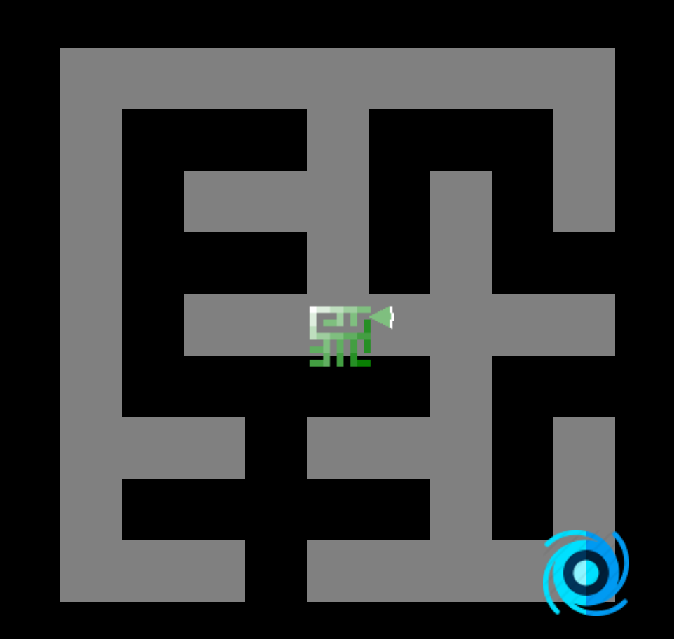
1. Here is our board.

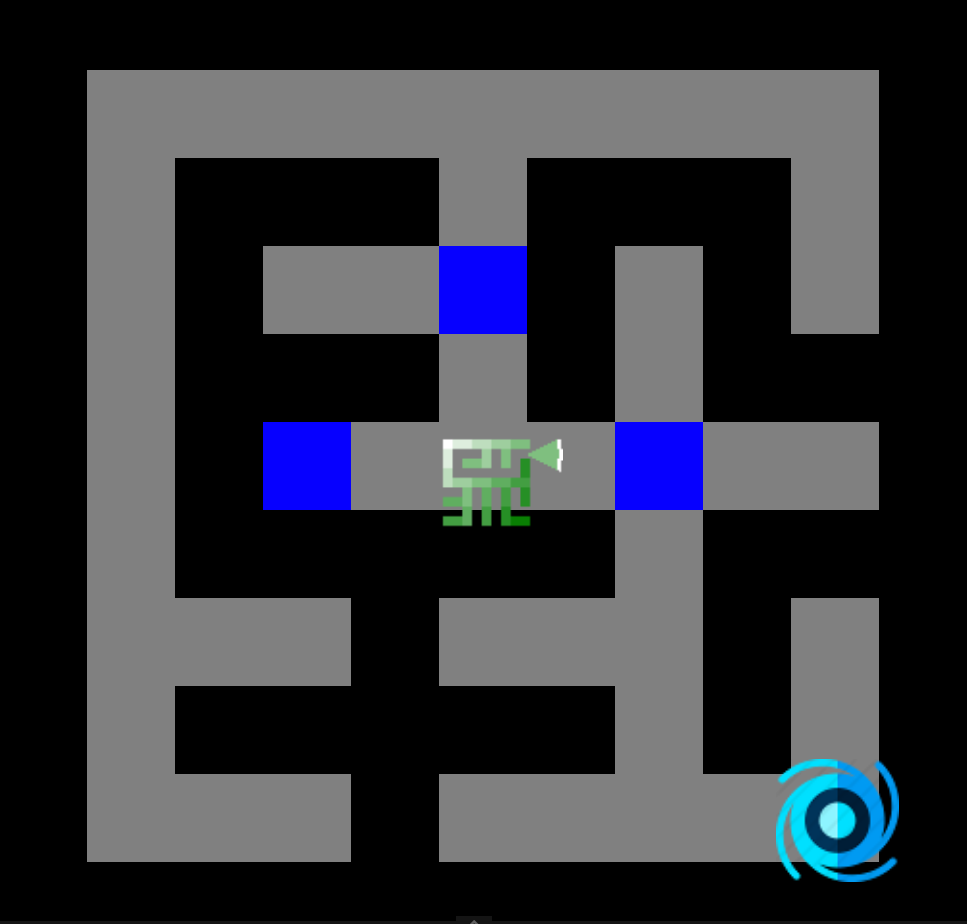
2. Examine all unvisited neighbors and add them to the queue. They are the closest nodes to the root (first circle, distance = 1).

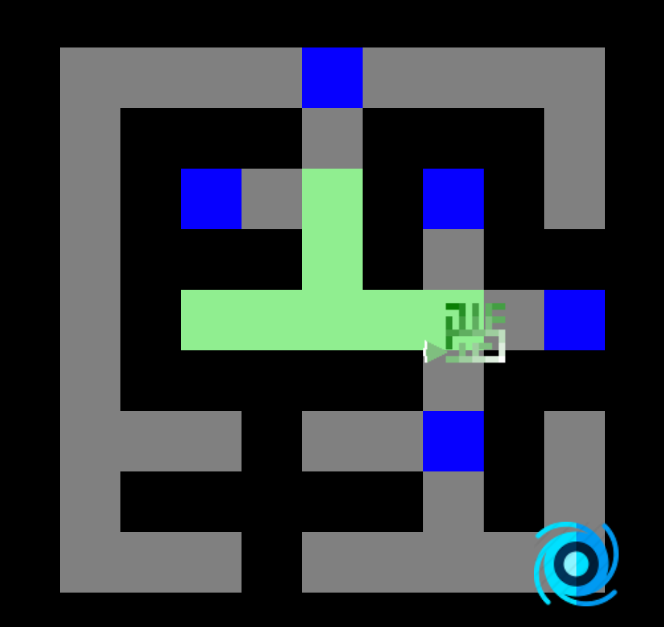
3. Each of the closest node will be examined first while adding their closest neighbors to the queue. This is the second circle (distance = 2) of the root (closest of the closest).

4. Here is the third.

5. Now the fourth.

6. Here we go : destination found!

Nodes in all the different directions are explored uniformly, appearing more-or-less as a circular wavefront (as the breadth-first-search) as we use a constant cost of 1 for all connections between two adjacent nodes.

Using a priority queue instead of a regular queue changes the way the frontier expands. Contour lines (based on distances) are one way to see this.

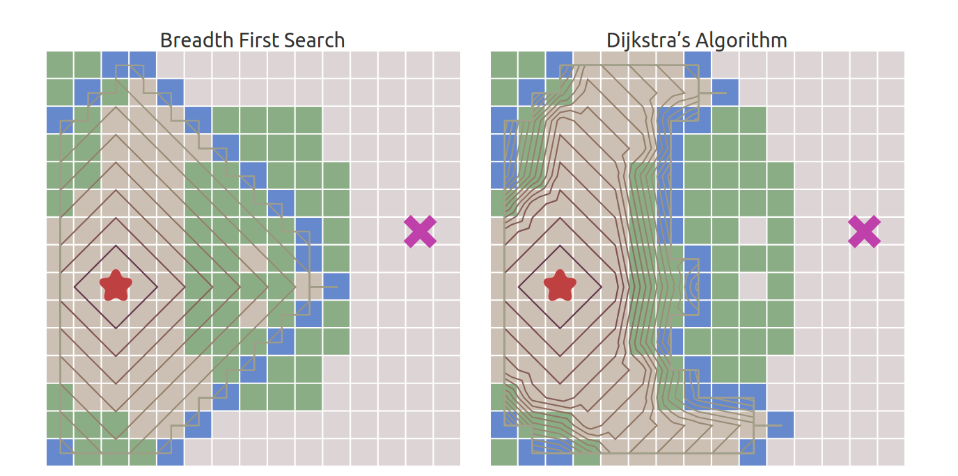
See how the frontier expands more slowly through the forests (source : redblobgames).