An adjacency list represents a graph (or a tree) as an array of nodes that include their list of connections. Let’s first see how it looks like with a graph and its equivalent adjacency list representation:

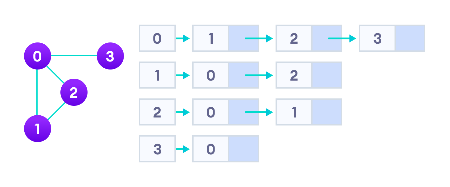
The idea is pretty simple : the index of the array represents a node and each element in its list represents an outgoing connection with another node. Easy to create, easy to manipulate, here is how the data could be represented in JSON :

[
  [1, 2, 3],
  [0, 2],
  [0, 1],
  [0]
] 

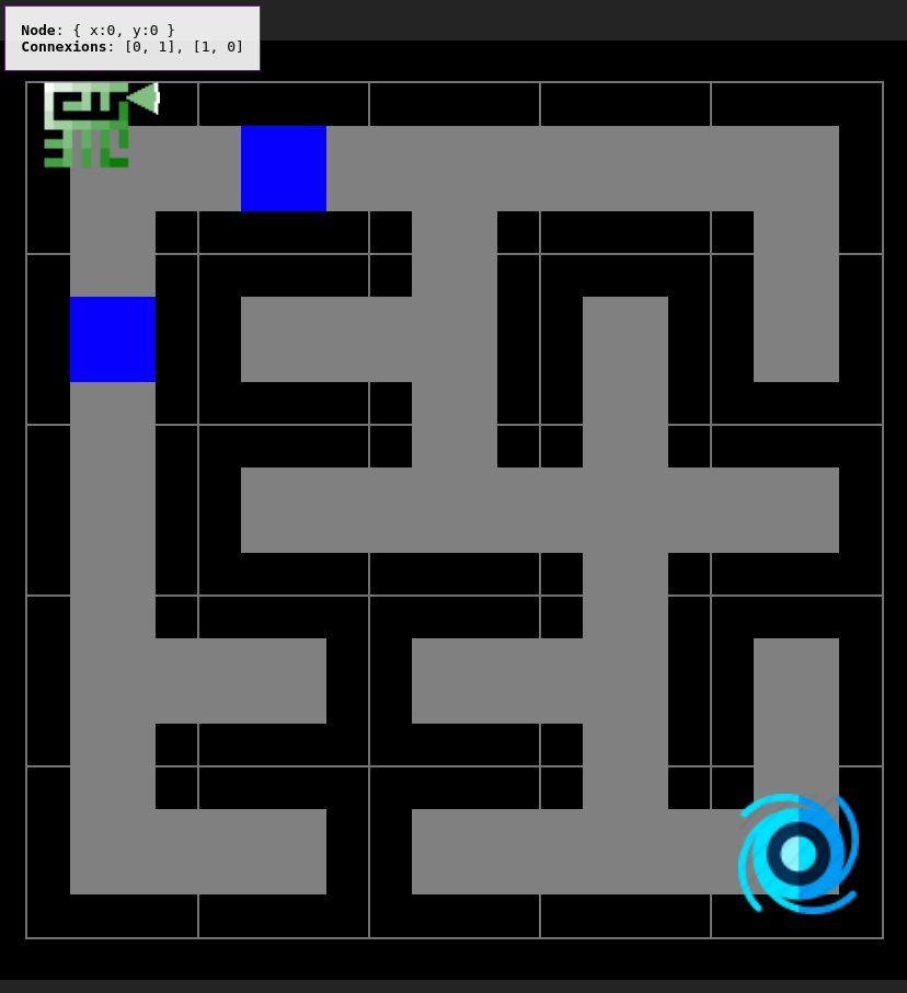
Yes, it’s that simple! It includes all the information we need to go through and to visualize graphs or trees. This is for instance the data structure we choose to handle our mazes:

Applications

The advantage of the adjacency list implementation is that it allows us to compactly represent a sparse graph. The adjacency list also allows us to easily find all the links that are directly connected to a particular node. It is used in places like: BFS, DFS, Dijkstra, A* (A-Star) etc.

Note: dense graphs are those which have a large number of edges and sparse graphs are those which have a small number of edges.

For a sparse graph with millions of vertices and edges, this can mean a lot of saved space.

Perfect, we know everything to create and manipulate our graphs!

Operate Adjacency Lists and Graphs.
Build our own structures.
Understand graph traversal algorithms.
Understand the advantages over an adjacency matrix.

What is next?

If you haven't jumped yet to maze generation algorithms, playing with them and using our explorer gives you visual insights of adjacency lists. We will soon study more graph data structures such as adjacency matrix which may be useful in particular cases.

To model this in C++, we can create a class called Node, which has two member variables:

- data: Any extra data you want to store
- neighbors: List of outgoing connections (using index as id)

  struct Node
  {
    Node(const T& data, set< int > connections) : data(data), neighbors(connections) {}

    T data;                // Any extra data you want to store
    set< int > neighbors; // List of outgoing connections (using index)
  };

  class Graph
  {
  public:
    Graph(vector< Node > nodes) : nodes(nodes);

  private:
    vector< Node > nodes; // All nodes contained in the graph
  };

Let's create a bidirectional graph!

  typedef Node< string > NodeT; // We choose to store the name's node

  auto graph = Graph({
                  NodeT("Globo", {1, 2, 3}),
                  NodeT("Whisky", {0}),
                  NodeT("Hybesis", {0, 1}),
                  NodeT("Boudou", {1, 2})});

Yup, that's it!
Great. Since we have all we need, let's define some useful methods.

  // Manipulations
  int Insert(Node node);                         // Insert a node
  void Connect(int idxA, int idxB, bool isBoth); // Add a connection between two nodes

  // Node Information
  int GetDegree(int idx);              // Return the degree of a node
  set< int > GetNeighbors(int idx);    // Return all the outgoing connections from a node
         

Manipulations

Insert / Connect

  // Insert a new node and return it's id
  int Insert(Node data)
  {
    nodes.push(data);
    return nodes.size() - 1;
  }

  // Connect two nodes together
  void Connect(int idxA, int idxB, bool isBoth)
  {
    [...] // Checks indexes validity
    nodes[idxA].insert(idxB);
    if (isBoth) nodes[idxB].insert(idxA);
  }
         

Quite easy, right?!

Node Information

GetDegree / GetNeighbors

  // Return the degree of a node (number of connections)
  int GetDegree(int idx)
  {
    [...] // Checks index validity
    return node[idx].neighbors.size();
  }

  // Get all outgoing connections of a node
  set< int > GetNeighbors(int idx)
  {
    [...] // Checks index validity
    return nodes[idx].neighbors;
  }
        

From this one, we can easily find out the total number of nodes connected to any node, and what these nodes are.

Let's finish the coding by implementing a graph traversal. We will use a simple BFS (Breadth First Search) strategy straight from our Graph definition.

  // We use the bool "isVisited" to keep track of our traversal
  typedef Node< bool > NodeT;

  BFS(int startIdx)
  {
    auto start = nodes.data()[startIdx];  // Get the start node
    start->data = true;                   // Set node to be visited
    Queue queue(start);                   // Put node in the queue

    // While there is node to be handled in the queue
    while (!queue.empty())
    {
      // Handle the node in the front of the line and get unvisited neighbors
      auto node = queue.pop();

      // Take neighbors, mark as visited, and add to the queue
      auto neighbors = node->GetNeighbors();
      for (auto it = neighbors.begin(); it !== neighbors.end(); ++it)
      {
        auto linkedNode = nodes.data()[*it]; // Retrieve neighbor node
        if (linkedNode->data) continue;      // Check if already visited

        linkedNode->data = true;    // Set visited
        queue.push(linkedNode);     // Add to the queue
      }
    }
  }
        

Voila ! You can code a GPS now.

What if I want to add some weights (distances)?

Adjacency Lists can also be used to represent a weighted graph. The weights of edges (links / connections) can be represented as lists of pairs:

[
  [{ "idx": 1, "weight": 4 }, { "idx": 2, "weight": 2 }, { "idx": 3, "weight": 0 }],
  [{ "idx": 0, "weight": 3 }, { "idx": 2, "weight": 3 }],
  [{ "idx": 0, "weight": 4 }, { "idx": 1, "weight": 4 }],
  [{ "idx": 0, "weight": 10 }]
] 

Try to implement this yourself as an exercise and try to find find the shortest path in this new graph. You may use a slightly modified version of our BFS algorithm seen above.

Adjacency Lists and Adjacency Matrix are the two most commonly used representations of a graph. Let's compare them shortly with:

- N the number of nodes.
- M the number of edges.
- degree(i) denotes the number of outgoing connections from node i.

Adjacency Lists
Memory space: O(N + M)
Check if two nodes are connected: O(degree(i))
Get all outgoing connections of a node: O(1)

Adjacency Matrix
Memory space: O(N * N)
Check if two nodes are connected: O(1)
Get all outgoing connections of a node: O(N)

For the most courageous, we will finish by seeing some trade-off between using STL’s vector, set, or list to represent the nodes (vertices) and the connections (edges). Let's first review some main differences:

Set
A set is automatically sorted
Insert/Delete/Find: O(log n)

Unordered Set
An unordered set is not sorted
Insert/Delete/Find: O(1)

Vector
A vector is not sorted
Insert/Delete/Find: O(n)

Linked List
A list is not sorted
Find takes O(n)
Insert/Delete: O(1)

Based on this, if you want to keep your edges or vertices sorted, you should probably go with a set. If you want a very fast search time, you should go with an unordered_set.

If find time is not that important, you can go with a list or a vector. But there is one more important reason that one might use a vector/list instead of set, which is representing multigraph.

A multigraph is similar to a graph, but it can have multiple edges between two nodes.